Fractals by nature are recursive and so is the way computers explore games to find optimal solutions! Using fractals, I wanted to create a way to illustrate how a computer may ‘see’ a game, to highlight moves it thinks are better than others. What I ended up with was not only a representation of what a computer sees, but also a visualisation of the game itself.

Fractals by nature are recursive and so is the way computers explore games to find optimal solutions!
Using fractals, I wanted to create a way to illustrate how a computer may ‘see’ a game, to highlight moves it thinks are better than others. What I ended up with was not only a representation of what a computer sees, but also a visualisation of the game itself.
Games can be very abstract and a lot of them won’t be applicable to this kind visualisation. However by focusing on grid-based games, like noughts and crosses and chess, it is possible to create these illustrations without sacrificing meaning.
In this blog I will explain how the visualisations are created, how they can be interpreted and what insights can be gained. The blog is intended as an overview and aims to give you enough background to understand what the images are and what they are trying to show. If you wish to know more, I am writing another post which will explore the process in more detail!
Starting simple

Figure 1
Take a game like Noughts and Crosses (aka Tic-Tac-Toe).
It is played on a 3×3 grid and player 1 starts by having a choice of 9 tiles.
As player 1, I want to know out of the 9 tiles to choose from on my first turn, which one is best? Phrased another way, which choice gives me the most opportunities to win? This can be quantified by the proportion of winning games to losing after choosing a tile.
For example, after picking a tile suppose there are only 10 possible ways for the game to be played after that point. Out of the 10 ways to play the game, 5 result in a win and 5 end in a loss. This would be a proportion of 5 : 5 or a 50% win rate. Another tile may have a 100% win rate where no matter how the game was played after the tile is chosen, player 1 always wins.
It is possible for a computer to calculate the win rate by checking all possible ways to play a game. However, for more complicated games, like chess or even simply increasing the grid size of our Noughts and Crosses game, the number of ways to play it increase exponentially. In this case, it is possible to approximate the win rate by taking a sample. Instead of checking every way, the computer randomly simulates a fixed number of games and uses that to make the calculation.
In figure 1, you can see an example visualisation which is coloured on a scale from blue -> yellow -> red. Blue represents no chance of player 1 winning (a win rate of 0%), a yellow colour represents an equal opportunity to win and to lose and the redder the hue the more likely player 1 is to win, if they chose the corresponding tile.
Since player 1 has an advantage by choosing first, no matter what their first move is, the win rate is always >= 50%.
One more time!

Figure 2
You can generalise this process and say you’ve looked to a depth of 1 – i.e. this is a visualisation of how many opportunities there are to win when looking 1 move ahead.
If you apply the same process to each of the 9 tiles in figure 1 you will be visualising to a depth of 2 (as seen in figure 2).
This ‘2-depth’ image is divided into 81 tiles (9×9 grid), each tile representing the first two moves that can be made in the game. E.g. the second tile (right of the top left tile) represents player 1 choosing the top left tile, followed by player 2 choosing the middle top tile.
The colour is then calculated using the same win – loss proportion, but starting from the second move in.
Handling illegal moves
You may ask, what the colour of the first tile represents? It is not possible for both the first and second move to be made in the same tile (top left in this case) so its position is an invalid/impossible state. I could have left regions of the image like this blank or coloured black. In a way I did leave it blank. If you look back at the 1-depth example (9 tiles) you will notice that the invalid tiles in the 2-depth are the same colour as the same position in the 1-depth. You can imagine first drawing the 1-depth image and then overlaying the 2-depth image, leaving the invalid regions transparent.
Repeat!

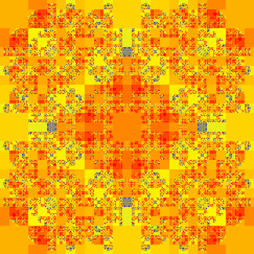
Figure 3: 1-5 depth visualisations
This process can be repeated again and again, provided there are still tiles to choose. However if you look at figure 3, there isn’t much different between the 4 and 5-depth images. In order to show the detail of higher-depth visualisations you can increase the image size. This is fine for relative low-depth images, but for every additional depth your image would need to be 3 times the previous one! If you were to render the entirety of Noughts and Crosses (9-depth) in full that would be a minimum of 19,683 (3^9) by 19,683 pixels! To put that into perspective, if you print this image at a resolution of 1 pixel = 1mm then the image would be over 19 meters across. Instead, we could keep the image at a reasonable size and use the same methods for rendering ‘infinitely’ zoomable fractals like the Mandelbrot set.
More than just a pretty picture


Figure 3: 3-depth
I am sure anyone familiar with Noughts and Crosses will know that the best places to go are the corners or the center. This can be seen in the visualisation as well where the corresponding regions of the image are more red, showing there are more opportunities to win.
In the 3-depth image (figure 3), there are also 4 distinctly blueish tiles. These represent the worst possible position for player 1 to be in after 3 turns. Try and see if you can work out what moves were played by examining the image.
Why a grid?

Grids offer a consistent layout which can be recursively applied to itself, which meets our fractal requirement. Noughts and crosses is a perfect example of this, as each tile can be divided equally into 9 at each step. As a result, regions of the image correspond directly to the same regions in the game’s grid, so even a pixel’s position has meaning.
Extensions
If Noughts and Crosses looks this good, imagine how interesting chess would look? If you are anything like me, you will be having similar thoughts, but one step at a time! With the process we have so far, it is possible to create all manner of cool looking images without needing to change much and it’s not just limited to games!
Visualising the 8 Queens problem
There is a famous chess puzzle which asks: How can 8 Queens (the piece, not the monarch) be placed on a chessboard, such that no queen is attacking another.
It turns out we can draw this too. Like with Noughts and Crosses it starts with a question: Where should I place my first Queen? Which tile gives me the most ways to complete this challenge?

Figure 4: Where should I place my Queen?
and again…

Figure 5: 2-depth

Figure 6: 3-depth
The question could be simplified by just asking if a queen can be placed in a tile at each step. This is synonymous with someone trying to solve this problem with brute force, placing each piece in a tile that looks fine until the ‘Oops’ moment when you realise this won’t work 5 moves in. This can be drawn using a grey-scale where the lighter the colour is, the more queens you were able to place before you’ve either won or realised it won’t work. The problem can also be generalised for any size of board and any type of chess piece…
Pieces’s board for a 3×3 and 4×4 board size respectively

Queen’s board

King’s board

Bishop’s board

Knight’s board


Rook’s board

Pawn’s board
Summary
There is a lot more I could talk about on this subject and I plan to, but I hope this has explained the core concept.
The idea of the project was to ‘see’ a game (turns out also puzzles) through the eyes of a computer, but really the computer is just a tool to explore the game in various ways.
Visualising games as fractals closely mirrors how we actually reason about them – looking several moves ahead is illustrated by recursively ‘peering’ into each move and seeing what the situation looks like. Using grid-based games allows for an implementation that easily lends itself to being drawn as a fractal, while visually still making sense for the ‘peering’ analogy.
Another analogy that I like to use is one of looking at the surface of a lake while divers explore the depth and bring up their finds. A blank image would be the lake’s surface and the algorithm used to explore the game would be the instructions given to the divers. In this way, it is possible to create animations of images being rendered in real-time, eventually showing patterns emerging from randomness as the computer performs more and more simulations.
In the next blog post I will talk about visualising one such ‘diver instruction’, the Min-Max algorithm, and how it is possible to visualise not just the game, but also how it is played.